Calibration example Linz
Introduction: calibration approach for the Lightmeter Network
Transferred to upgraded wiki --GW (talk) 18:21, 30 July 2014 (CEST)
The Lightmeters, as any sensors, generate a signal as "counts" in an instrumental system. The counts are determined by the signal, the sensor-properties, the amplifier and the analog-digital converter. The "counts" need to be converted to numbers relating to a physical unit by means of a standard. Because the Lightmeter network is global and aims to monitor long-term changes of the night sky brightness, a globally accessible standard is needed that allows repeated checks over a long period of time. Therefore, one has to ensure
- a homogeneous calibration of the network to inter-compare the different stations, and
- a repeatability of the calibration in order to monitor any degrading effects of the detectors sensitivity caused by, e.g., aging effects.
Following a suggestion by Jan Hollan (What is Light Pollution? by Jan Hollan ) to relate all light-pollution effects to the Sun, as the primary natural source of light, the calibration strategy is to use
- the Sun,
- the Moon, and
- the twilight,
as secondary calibration references (the primary being the one used in the definition of the respective SI units).
The Sun is stable down to a level of a few permille, thus better than the measurement goal of a long-term accuracy at the percent level. The brightness of the Moon depends from its apparent position to earth as well as on its albedo that is supposed to be stable over Millions of years. The twilight is also found to be relatively stable, in particular, the late twilight that is controlled by atmospheric layers above the Tropopause, i.e. layers at more than approximately 8 km height, where no influence due to weather is expected. Atmospheric effects can be controlled and bounded by meteorological and other astronomical studies (e.g. daylight total radiation measurements and the classical astronomical extinction determinations).
To use the Sun, the Moon, and the twilight we need models that calculate their effects for a given site, i.e. position, height and atmospheric conditions. That involves two steps.
- to calculate the Sun's and Moon's apparent positions and
- their total radiation and corresponding brightness.
- For the calculation of the positions I use high precision ephemerids in the pyephem implementation.
- The Moon is calculated by using a phase function described by Kasimir Graff, Handbuch der Astrophysik 1958,p 400.
- Extinction is determined by calculating airmass according to Rozenberg, G. V. (1966). Twilight: A Study in Atmospheric Optics (New York: Plenum Press), translated from the Russian by R. B. Rodman, p. 160. and assuming a zenital extinction (at airmass 1) of 0.23 mag. The Rozenberg airmass has the convenient property to lead to a reasonable airmass of 40 at a zenith distance of 90°.
- The solar total radiation model is used as put together by Duchon and Malley 1999 Journ. Appl. Metr. 38, 134.
- The modeling of twilight (Sunset/Sunrise down to h_Sun = -18°) is done using the table in Siedentopf and Scheffler in Landolt-Börnstein, Gr IV, Vol. I, sect 1.5.3., p.60, Springer 1965.
Checks with measurements obtained on Paranal confirm these models to certainly better than 10%, most likely better than 5%.
Is there a 'general' atmospheric extinction model included?
- extinction for the astronomical part is done via airmass + zenith extinction.
- the total radition model implicitely produces an exctinction model because it tries to account for typical radiative transfer through the clear Earth-atmosphere parametrised by meteorological input.
Search for a clear day and night
The models matches best the observed Sun and Moon brightness for altitudes of at least 30° above the horizon, so far. For the twilight, a diffuse illumination of the clear sky is best, i.e. when the Sun has set and is significantly below the horizon so that the light is dominated by the upper atmosphere.
In short: for calibration a clear day, night and twilight is optimum.
The Sun serves to calibrate the daylight part of the Lightmeter with its non-linear characteristic. The twilight brightness reaches from the high daylight values to the faintest values of the measurements at the starlight level, thus assuring calibration of all of the many orders of magnitudes the instrument covers.
The day-signal reaches a kilowatt per square meter (kW/m²) whereas starlight is in the 0.01 milliwatt per square meter (mW/m²) domain. The twilight also connects the daylight part to the very sensitive night-time part where the Lightmeter shows a linear characteristic, sensitive to below the faintest natural outdoor light levels. By natural outdoor light levels we mean those of skies with and without overcast, as well as reduced light-levels in canons where only small fractions of the sky contribute to the natural illumination. The Moon in a clear night, with its characteristic brightness does not cover so many orders of magnitude but gives very important constraints. It is used as a check / cross-calibrator? here.
Thus we need a clear day with the Sun preferable above 30° height for an accurate calibration. The daylight part of the Lightmeter connects the measurements to the absolute values of the solar radiation (solar constant) and thus the Sun high up in the sky is needed for best accuracy for the absolute values of total radiation (energy flux through a horizontal unit surface) measured in Watt per square meter, W/m².
A clear evening- and, if possible, morning-twilight assures the correctness of the calibration at the night levels.
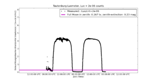
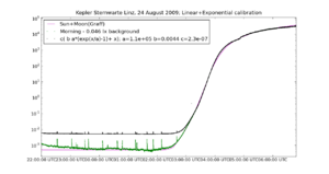
In Fig.1 the August measurements are plotted for the Lightmeter L3 at the Kepler observatory in Linz, see Kepler-Sternwarte Linz. It is one of the the first stations that was installed an running outside of the Lightmeter development team and provides the longest set of measurements uploaded to the Lightmeter database. The selection of August resulted from a search of the entire dataset from March to December 2009, computing the residual/standard deviation over a moving 20 min window of the raw data and visual inspection. August also assures the Sun to be close to maximum height (at Linz) at noon.
In the figure three lines are plotted: The black dots that connect to a line are the measured counts by the Lightmeter multiplied by 2.E-6, a rough estimate for a conversion to Lux-values. The Lux is the SI unit of illumination and irradiance. This is for a better comparison to the calculated values for the Sun (magenta line) and Moon (blue line). The day-night variations are clearly visible in the black line of Lightmeter measurements and the theoretical Sun. Also clearly visible is that the instrumental counts fall systematically short of the theoretical Sun during daylight. These is the consequence of the non-linear behaviour of the instrument for conditions brighter than about the full moon. The flat daylight parts are the hallmark of the sensor's non-linearity at high light levels. For lower values (twilight and down) the instrumental counts follow the Sun until some lower limit that is determined by the night-sky brightness after the end of the (astronomical) twilight - that lower flat part in the linear regime of the sensor is marches with the model (magenta line) except for a constant factor (constant upward shift in the log-plot) before calibration and due to starlight, moonlight or light-pollution contributions from artificial light sources.
For the moment we are not interested in the details but to look for a nice smooth part of the curve, where only the Sun, Moon and twilight contribute to the signal and not weather effects like absorption (decrease of light) and scattering (increase of light) by clouds are visible. The basic rule: the smoother the curve the less weather-effects that typically cause short-term-variation are present. (Beware of the fog).
Looking to the August data we find a smooth part on August 23rd to 24th that contains a smooth daytime part, a smooth twilight and a smooth very low night-time part. There are other clear parts in the curve but not as continuous over the twilight and not as smooth.
Maybe this statement should be connected with the RMS values to get a threshold for clear/cloudy and if it therefore can be used for calibration:
- RMS-values of less than 0.02 for the relative variations generally correspond to excellent conditions. A threshold near 0.04 will include some weather and larger variations combined with the systematics in weather will very likely degrade any calibration to below 5% accuracy.
Check your data
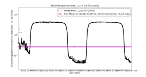
To make sure Aug 23rd and 24th are suited for calibration,we have a closer look at the two days and nights in the next Figure (2). It shows a blow-up of figure one with the data of Aug 23rd and 24th cut out and now plotted with their full 1Hz sampling. The variation and smoothness are much clearer now and this check confirms the suitability of the selected data.
The flat daylight parts are now more obvious as well as the qualitative aggreement between the instrument counts and the models at twilight and night.
Try a logaritmic plot
Because the brightness range of natural light is so large (8 orders of magnitude, a factor of more than 100 Mio, Sun to night sky) it is very useful to use a logarithmic plot to inspect the measurements. A plot with linear axis shows the measurements with the value plotted on the vertical axis proportional to the measured number. Thus a double value is at double height. 1 cm corresponds to a given constant amount, the scale of the plot. In a logarithmic plot the same distance corresponds to the same constant factor. Thus 1 cm on the figure does correspond e.g. to a factor of ten. 2cm to a factor of 100, three to 1000 etc..
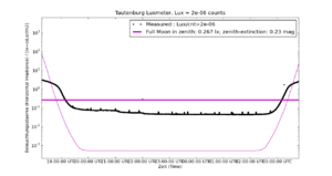
The same data that are plotted in Fig.2 using a linear scale, are plotted logarithmically in Fig.3. As we move downward from the maxima at the top of the figure we always move down by a given factor. We first see a similar thing as in the linear plot. The first factor of ten looks similar as in linear figure 2. The second factor of ten still can be followed in the linear plot but the twilight values near the magenta line for the full moon in zenith are near zero and can hardly be seen. The logarithmic plot allows to follow the variations into the night --- down below the magenta line --- and also during the night-time minima. Thus night-time variations caused by clouds can be easily identified. In our case the night-time level is very smooth, except for shorts spikes connected to the steel production of Linz's industry.
With the smooth daylight and twilight and no apparent variations during the night we confirm the selection for calibration because no cloud-induced variations are visible. Numerically, the RMS-variation values in a (20min) window remain small.
The spikes are present every night in Linz and we will try to avoid them during the calibration procedure. Because of their short-term nature, there effect will be limited in any case if we use as sufficiently large amount of data.
Check for time or longitude offset
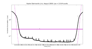
Once you identified a period of clear skies for calibration, have a look to inspect it for plausibility. This is done in Figure 4 by comparison to a model of the Sun, twilight and night-sky brightness. Ideally the twilight should be symmetric and in the lower part, where the Lightmeter-sensor is linear, only show a constant vertical offset (corresponding to a constant factor in the log plot).
In Figure 4 the black measurements are not centred to the magenta curve of the theoretical twilight. Thus at the same height/depth of the Sun relative to the horizon there are different brightness measurements recorded. The black line appears displaced to the right relative. That is typically due to an error in the longitude of the site used for the ephemeris calculation or to a clock error. The clock error may be due to a wrong UTC-offset (wrong time-zone, error in daylight saving time) or an inaccurate clock.
Correct a time-offset
We identified the shift as a time-offset in the Linz-data an corrected that by subtracting a clock-error of 180s.
Correcting the clock to a about 1s accuracy is essential for the calibration using the twilight, because the light levels drop very fast during civil and nautical twilight. Any time error will translate into a calibration error.
The check and correction is always possible to good accuracy because of the symmetric nature of twilight and rise/set phenomena.
Maybe link to Google Maps to retrieve reasonable geographical coordinates:
Select a piece of data for calibration
Motto: The smoother the better. Because smooth means clear most of the time. Note: In a logarithmic plot typically relative variations to 1% percent times the number of displayed magnitudes are visible. So a smooth-looking curve in our context contains small time-scale variations of at most 2%.
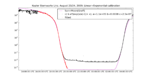
We next look at the evening twilight of August 23rd in a zoom displayed in Fig.6. Detailed inspection shows some daylight variations before 15:30 UTC, likely due to cloudlets. Also the spikes due to the steel production are visible during the astronomical night (after 20:00 UTC). Near 21:10 UTC there is a step-like decrease, likely due to the switch-off of some lights. Actually Linz switches off half of the public lights at 23h local time (CEST). That and the flatting near 20:00 is indicative of the approach to a "background" level (light pollution) that we should not use for the calibration. To keep the influence of light pollution or any other background on the calibration as small as possible, we should only use the data somewhat above that level for calibration, so that any perturbing effect is not dominating the signal. We select only data about a factor of two above the background so that any light-pollution should contribute less than 50% to the signal.
The red curve shows the final selection of the calibration data. It avoids the cloudy time earlier in the day, a close approach to the light-polluted background at night and most of the steel-production spikes.
We will proceed with the data marked red in Fig. 6 for the calibration.
Calibration to theoretical twilight with linear and exponential part
The basic properties of the sensor of the Lightmeter are a linear low-level part and an upper non-linear part with a logarithmic behaviour. The transition occurs by design near the full-moon level. See Lightmeter - instrument properties for some more details and measurements.
To convert the sensor output to physical units we model the two parts by a combination of a linear and an exponential part. The latter inverting the logarithmic daylight behaviour. The form of the linear part is straightforward,
y = c x
To make sure the exponential part linearly goes to zero for small values, we use exp(x)-1 because it goes like exp(x)-1 ~ x for x << 1. We allow for a scale parameter a to adjust the transition from linear to exp, thus
y = a exp(x/a) - 1
the factor a to get keep the behaviour like x at x << 1. We add a proportionality, b
y = b (a exp(x/a) - 1)
to scale it relative to the linear part. Putting all together we get the following form of the conversion relation
y = c ( b (a exp(x/a) - 1) + c x = c ( b (a exp(x/a) - 1) + x ).
a,b,c are the parameters that have to be determined by fitting the above relation to the data.
Many sensors are located at light-polluted skies. Hence the natural light is superimposed on a background of artificial light. Thus to remove that background as a consequence to be able to follow the twilight longer (ie to smaller values) is useful. Therefore we fit the data to the above expression plus accounting for a constant background x0.Thus the form before the fit looks like.
y = c ( b (a exp(x/a) - 1) + x ) + x0
x0 is light that is present independent of Sun, Moon and twilight - the artificial light.
The fit for a possible background (light pollution) is necessary in all areas that have dominant artificial sky brightness, but is also convenient to remove any perturbing lights. Nearby street-lights reflecting via trees, buildings, the neighbour's Christmas-lights for example. As long as they are constant they can be removed successfully. This is particularly important at bright sites were otherwise the calibration would only rely on the upper light-levels and possible not connect to the linear part. E.g., if the skies are always brighter than the full moon.
The result of the fit is displayed in Fig. 7. Again the data used for the fit are plotted in red. Now the results are plotted with the values a,b,c and x0 as determined by minimizing the quadratic differences between the data and the model-function (least squares fit). The red curve shows
y = c ( b (a exp(n/a) - 1) + n ) + x0
where
n are the numbers (counts) measured by the Lightmeter
and
  a  = 1.067e+05,  b= 3.752e-03,  c= 2.479e-07
  X0 = 9.86e-3
Thus the red curve shows the measurements calibrated to the natural light (magenta) with the background x0 subtracted. That background is the mean artificial light present during the calibration time. Note that the twilight can be followed and fit to a level of below 1mlx, the natural night-sky brightness, despite the fact that there is a significant background of artificial light.
The black curve is the calibration applied to the measurements, that is without subtracting the background:
y = c ( b (a exp(n/a) - 1) + n )
again with
a = 1.067e+05, b= 3.752e-03, c= 2.479e-07
That represents the actual situation measured. Because the model expressed the light-levels in Lux the direct application of the obtained fit puts out values that have the physical unit of [Lux], the SI-unit of illumination.
Comparison to a fit to the morning twilight

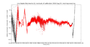
Inspection of the daylight measurements made in Linz shows an asymmetry between the morning and the afternoon. That is attributed to the Sunlight crossing the city and the large industrial area with its aerosol and water-vapour. Because that causes a shape of the typical morning Sunlight that is not represented well by the model and leads to systematic differences we use the clearer situation in the afternoon, despite the fact that the city itself is darker in the morning twilight.
But for a comparison we show the fit and give the resulting data for reference and to estimate the uncertainties that may be caused by similar effects elsewhere.
The fit result for the morning are:
a = 1.094E+5 b = 4.374E-3 c= 2.337E-7
The linear coefficient c in that case is 6% smaller then for the evening/afternoon. That is caused by the differences in the daytime part (extra brightness around about 10h local time) by extra, apparently scattered Sunlight. Possibly from industrial vapour clouds or aerosols.
With a background X0 of
X0=4.74 mlx about 48% of the evening value
Thus the after-midnight (maybe 23 local time?) skies in Linz benefit from a cut in half of the light-pollution during the night.
Check fit and compare to total radiation model
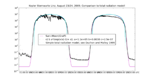
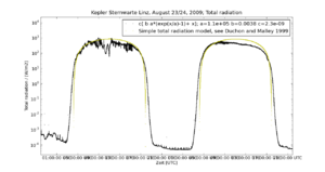
To convert the measurements to total radiation in Watt/m2 we compare our calibrator, the model for the Sun, to a the simple total radiation model put together by Duchon and Malley 1999 Journ. Appl. Metr. 38, 134. See Fig. 8.
By fitting the maximum of the solar model brightness to the total radiation model we obtain the conversion factor from Lux to W/m² applicable for our situation. Thus it is implicitly assumed that we can calculate the solar total radiation near maximum height from the simple total radiation model. This fit results in a correction of 7% with respect to a geometric calculation with our assumed zenithal visual extinction of 0.23 mag.
The fit to the total-radiation model to the one of solar illumination is good for sufficient height of the Sun (5 UTC to 17 UTC). The cyan curve of the total radiation model covers the magenta curve of the solar illumination model. On Aug 23rd the overall shape of the measurements also reproduce the model in spite of some variations due to clouds. At lower Sun height the total radiation model fails to fit the data, a well known effect of such simple models. On the 24th the typical asymmetric behaviour of the total-radiation (increase before noon when the Sun shines over the city) in Linz is visible. The total radiation model fails to fit the measurements. This is often seen in the Kepler-Sternwarte data and is the reason to calibrate with the evening twilight where the models fit better.
That it is the city and not a reflection from the dome of the Kepler-Sternwarte - the sensor is mounted to the south-east of the dome, the city centre lies east of the sensor - is corroborated by the fact the December measurements that have the Sun more towards the S do not show the asymmetry. The Dec measurements have been rejected for the calibration because of the lower Sun leading to larger uncertainties via the application of the total radiation model at high air-mass (low Sun-height), where it is uncertain as seen in Fig. 8.
Convert to total radiation (W/m²)
Matching the total radiation model near noon leads to a conversion factor of
1/109.3
from Lux to Watt/m².
The simple value obtained by dividing the Solar Constant of 1367.0 W/m² after applying a zenith extinction of 0.3 mag and 129000 Lux for the Sun in zenith would be 1/116.3. Thus the total radiation model gives 6% correction to the simple geometric estimate based on standard values.
Note: the situation is better than that because of the assumption of 0.23 mag for zenith-extinction and 0.3 for the estimate. The ext-difference is
  In [6]: 116.3*2.51**(0.23-0.3)
  Out[6]: 109.04
Assuming that the total radiation model is significantly better than the simple
estimate the resulting error should be significantly less than the 6% correction.
An overview over the obtained calibration is shown in Fig. 9.
Check with moonlight and clear days and nights
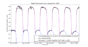
With the calibration completed we check the correctness of the model by looking at other references not used in the process. The simplest thing is to use the Moon for that purpose. Errors in the Moonlight would most likely come from the phase function or the airmass and extinction calculation, that is independent of the one in the total radiation model.
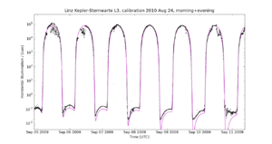
Figure 10 shows a few clear nights with Moonlight in Sept. The Moon (with the Graff phase function, see above) is plotted in blue. The natural light (Sunlight+Twilight+Moon) in magenta. If the weather is clear (no short time variations), from Sep 6 to 9 the black measurements fit well with the Moon and the natural light. As the moon wanes and fades an offset becomes visible that is due to the background of the city lights, enhanced by some cloud on Sep 10th.
Thus the Moon confirms independently the obtained calibration.
Use of the Moon will be improved by using Kieffer et al. 2005 (phase and libration dependent albedo) that has been worked out to develope the Moon as a calibration standard for Earth observations.
A day and night calibration for the L3 Lightmeter at the Johannes Kepler Sternwarte in Linz
Station page: Kepler-Sternwarte Linz
X = c ( b (a exp (n/a) - 1) + n )
   n ... counts (sensor output)
   X ... physical quantity (total radiation in [W/m²] or horizontal illumination [Lux])
  a = 1.067e+05,  b= 3.752e-03,  c= 2.479e-07    Lux
  a = 1.067e+05,  b= 3.752e-03,  c= 2.268e-09    W/m²
Improved calibration accounting for daytime sensor warming
The calibration shown above shows some asymmetries near the maximum brightness and during daytime, in particular on the clear day used for the calibration. For the Lindenberg-Lightmeter a temperature dependent-term has been introduced that accounts for the small temperature dependence of the solar cell (0.3 %/°C). A check with independent measurments of total radiation at Lindenberg confirms that the extra term improves accuracy during daytime. Here we apply this new term to investigate Linz measurements and improve the accuracy of the Linz calibration.
X = c ( b (a exp (n(1+dT)/a) - 1) + n )
   n ... counts (sensor output)
   X ... physical quantity (total radiation in [W/m²]
         or horizontal illumination [Lux])
  a = 1.2835e+05,  b = 1.6468e-02,  c= 2.5778e-09  d= 3.4726e-03 W/m²
  a = 1.2835e+05,  b = 1.6468e-02,  c= 3.1887e-07  d= 3.4726e-03 Lux

  Background X0= 6.741 mlx
Conversion factors determined from total radiation model
  Watt/m² --> Lux       109.30
  Lux     --> Watt/m²   0.008084
  c_Watt = 2.57776395614e-09
  Log:
  SJD0=(2009,8,24,2,12)    to (2009,8,24,2,19)
  SJD1=(2009,8,24,2,22)    to (2009,8,24,2,51)
  SJD2=(2009,8,24,2,41,46) to (2009,8,24,17,00)
  SJD=SJD0|SJD1|SJD2
  In [656]: Y.fit_em1_to_natLight(JD_select=SJD
             ,type='em1c0T',Lux_range=[0.0001,300000])
  Out[656]: (array([1.28351951e+05, 1.64679802e-02
                  , 3.18872335e-07,-6.74090159e-03, 3.47259838e-03]),1)
   plot_date(Y.JD-.pylab_JD0
            ,Y.Sunlight_Watt_per_square_meter_from_JD_DM(Y.JD
                 ,surface_pressure=953.0
                 , T_dew_C=10.0)*0.94/X.Watt_per_square_meter_per_Lux
                 ,'c,', label='DM model,P=953.0/T_d=4/k=2.78')
Test query to Lightmeter database at GVO
For calibrated L3 Linz Lightmeter data in March to December 2009
Test query at GVO - to plot data scroll down and select VOplot as format
Notizen an Raab
nach Email an Herbert Raab
Anbei die erste Auswertung der Linzer Messungen mit voller Kalibration. Das ist auch die Kalibration für die GVO-DB (CC an M. Demleitner).
Die Kalibration (Sonne und Dämmerung) mit Umwandlung auf W/m² mit einem Globalstrahlungsmodell.
n ... counts (Ausgabe des Sensors) X ... phys. Größe W/m² (oder Lux)
   X = c ( b ( a exp n/a - 1 ) + n )
   a = 106691 b = 3.752E-3 c= 2.268E-9    [W/m²]
Zur Orientierung in Lux
   a = 106691 b = 3.752E-3 c= 2.479E-7    [Lux]  X0=9.86 mlx  abend
  (a = 109401 b = 4.374E-3 c= 2.337E-7)          X0=4.74 mlx  48% abend
                              -6%
Alle Fehler etwa 5%.
X0 ist der im Fit ermittelte Hintergrund. Das ist die Lichtverschmutzung unter besten Bedingungen. Bei Euch ist der Hintergrund/LV am Morgen ziemlich genau halb so groß wie am Abend. Einfachste Interpretation: genau entsprechend der Halbschaltung.
Die Grafiken für die Verteilungen anbei. Es sind 1/10 aller Messungen (insgesamt rund 20 Mio) weil dass mein Netbook noch vernünftig (in ca 30 Min) schafft.
Die W/m² "Globalstrahlung" (wie bei der "Solarkonstante") werden die prim. Messgröße, die Lux nur zur Illustration. Wir messen genau die Globalstrahlung wie in der Meteorologie nur eben bei Nacht.
Die Kalibration ist auch am Tag sehr schön, und wie bekommen als Nebeneffekt die erntbare Solarenergie.
Ich habe begonnen die Kalibration auf der Wiki zu beschreiben und mache das in den nächsten Tagen fertig, aber grafisch sollte man schon nachvollziehen können wie das klappt. http://kuffner-sternwarte.at/hms/wiki/index.php5?title=Calibration_example_Linz
--GuentherWuchterl 23:28, 11. Feb. 2010 (UTC)

